
Filter synthesis objective functions with Differential weighting (Heavi)
For a long time now we have known ideal mathematical solutions for determining the inductance and capacitor values of networks to realise low-pass, high-pass, band-stop or band-pass filters with a given desired behaviour. These methods often require a rigid fixed structure in order to associate analytical solutions to specific component values. The Chebychev and Butterworth prototype filters are a great example of this. For more intricate structures one can try to derive component values for elliptical filters.
Another approach might be to use optimisers to find component values required to realise a specific filter performance. Now in practice this methodology is rarely used because most of the times our prototype filters work sufficiently well.
In some circumstances however we wish to integrate some filter performance through the use or perhaps abuse of parasitic component values or other structures to realise filtering behaviour separate from well defined ladder networks. In this case an optimiser may be able to assist us to find component values that will satisfy our requirements.
The key challenge with optimisation algorithms is often finding an appropriate objective function. The objective function is a function that maps a certain scalar value to our trial solution (often just an array of component values) as some sort of multi dimensional scalar mapping. The optimisation algorithm then tries to find the values that will minimize the objective function.
It is known to most that the easiest optimisation algorithms such as Gradient Descent can struggle to avoid local minima. These are solutions where any marginal change to a component value will always make the performance worse. I emphasised the word performance for a reason.
The performance is literally defined by our choice of our objective function and this choice of objective function plays a crucial role in the success of our optimisation algorithms. If our objective function rates certain “bad” filter performances as marginally worse than the optimal one, we can’t expect our optimiser to find the global optimum, even if there are multiple.
A solution to this problem would be to just search the entire component value space for our global optimum, but with larger networks this space may be so large that one can not reasonably find an optimum in a finite amount of time. Especially because component values used may span multiple orders of magnitude. For global optimisation in large multi-dimensional systems there are other algorithms that attempt to find a good solution in a fairly limited amount of time. Even for these algorithms, setting a proper objective function is crucial.
In this article I will explore a possible realisation of objective functions for filter synthesis that utilizes a concept I call differential weighting.
The trial case
In our example we will consider a simple Low-Pass filter with the following masks:
DC - 3GHz: S11 < -15dB
3.5GHz - 5GHz: S21 < -30dB
5GHz - 10GHz: S21 <-20dB
Please note here that his test case is just artificial which tries to illustrate a point more so than being practically useful. I also set the requirements such that a solution exists with the chosen topology that can satisfy these requirements.
As a filter topology we will a low-pass elliptical filter as a basis.

The topology of an elliptical filter (low-pass).
We will define our objective function now by considering the two frequency regions.
Setting an objective per frequency region
For the first region up to -3dB we want our S11 to be below -15dB. An easy way to compute this objective function is to compute the S11 for this region at a given number of frequency points and then subtract -15dB from it. If our S11 is greater than -15dB this value will be positive and otherwise negative. We can then clip our value to be 0 for all values below 0 such that this objective function returns 0 if and only if the S11 is below -15dB at a frequency point.
We can do the same for the S21 component for a given set of frequency points above 3GHz up to 10GHz.
The first point now is that we have an objective function for each frequency point within each region and not a single one (which we need in order to optimise). We thus need a way to “weigh” our objective function.
Sticking within our first pass-band region, we can consider 4 common ways of combining all our objective function values at each frequency point.
Minimum value
Average value
Root-mean-square value
Maximum value
In this case the minimum value sees no obvious utility because its not that hard to have one frequency point be below our limit, we need all or at least most of them to be. All the other metrics ensure that the objective function is only zero if it is at all frequency points. The question then becomes which one is best.
All of these options are in fact a member of the more general concept called a “general mean”, a power mean or the Hölder mean (link). These generalised averages are based on the concept of Lp-spaces which implement a P-norm.
In our Cartesian world, the “measure” of a 3D coordinate is the square root of the individual coordinates squared and added or: D = √(Σ c²) where c is one of the x,y,z coordinates. We can in fact extend this concept to N-dimensional spaces. The so called Manhattan distance is just the sum of the coordinates: D = Σ |c|. Its not hard to see how these two metrics are specific instances of the following metric: D = (Σ c^p)^(1/p) where the Pythagorean metric corresponding to our world is that where p=2 and the Manhattan distance that where p=1.
We can consider this way of “measuring” distances as analogous to different forms of averaging that normalise this distance to the dimensionality of your space. In this case the normal average mean = (Σ x)/N would be the average variant of the p=1 norm and the root mean square: √((Σ c²)/N), the average variant of the p=2 norm.
We can also see how in this generalised mean concept puts more emphasis on extreme values for higher values of p. It is in fact true to say that the p=infinity norm is equivalent to the maximum value of our set of numbers.
In any case, we may choose any arbitrary P-norm between 0 and infinity (large values are not advised for floating point arithmetic) to measure our objective function and we may find that P-norms of 2 or greater work well as they are just the right amount of sensitive to very narrow regions where our objective function becomes large.
It is often not good to choose the maximum-norm because it has a tendency to mess with the continuity of our N-dimensional objective space. Because in this case our S-parameters have an upper limit, the maximum norm may be constant for a large region because it looks only at the largest occuring value. Even non gradient-based algorithms often use some assumption of proximity when searching for optimums. They just don’t directly compute a gradient.
For the sake of the rest of this article, i’ve found that for this specific problem, something between a P=2 norm and a P=4 norm works well.
Once we have this implemented we are at a next problem.
Setting a global objective function
At this point of our analysis we have an objective function value for each frequency band that measures how “bad” our filter is effectively. A value closer to 0 means that our filter is closer to our final requirement. The problem now is how do we combine these two metrics to form one objective function value?
We could simply repeat the previous process and apply an p-norm with a p-value of our choosing, an average or RMS norm seems appropriate. When we try to synthesise our filters however we will find that often, good filters aren’t found. We can quickly see based on our results why this is.
A failed optimization (differential evolution with a pop-size setting of 10)
In our example we use differential-evolution as our search algorithm (these work reallywell). We must note at this point that that differential-evolution is a non-deterministic algorithm which means that sometimes when we run it, it works and sometimes it gets stuck such as in the case above.
The problem we find ourselves is that a large portion of all possible filters (with bounded realistic component values) will either completely block or completely let through the signal in both frequency regions. In the case above we have a full rejection for all frequencies. These solutions are fairly simple to find because they lie at the extremes of our search space and occupy a fairly large portion of it. Any filter where the first capacitor is very large will almost always stop all frequencies.
Because of this, small variations of the other components will not move these filters to anything with better performance and thus the optimizers have a tendency to “get stuck” at these local minima.
We thus need a method for our search algorithm to learn that some changes to the filter values are better even if we make it stop working well in the desired stop band.
To solve this problem I introduce the concept of differential weighting
The solution
Lets consider the case where our optimiser is stuck at a component value set where there is a stop-band everywhere.
The idea of differential weighting is to add a value to our objective function that measures the difference between the largest value of our objective function values and the smallest and then compute the difference. Then it may raise that difference to some high power, say 5. If we have an array of objective function values x, the objective function would change from
O(x) = Pnorm(x) to O(x) = Pnorm(x) + a*(max(x)-min(x))^n
In cases where our filter optimiser gets stuck in these local minima, we are in a region where one objective function is 0 (in this case for the stopband because it satisfies the requirements), while the other is some large value, lets say 10. In the case where it is 10, the difference is now large which drastically increases the total objective function value.
If the optimiser can make a change to the filter that improves the pass-band performance at the cost of the stop-band performance. Previously that would have increased the objective function in both regions which means that it wouldn’t have been considered as a better option. With differential weighting, the improved passband performance and worsened stop-band performance actually brings both values closer together which means that the differential weighting decreases quickly. This improves the likelihood of finding a global minimum if it doesn’t get too dominant around the global minimum.
The disadvantage of just having this differential weighting is that depending on how strongly you add this weighting to the mix, the optimiser may start to prefer realisations where the pass and stop-band performance is equally bad or mediocre. It may thus find a small local minimum where no deviations are allowed because it upsets the differential weighting too much to find another lower local minimum.
To fix this we added the exponent. What this exponent does is that it flattens most low values for our differential weighting to 0 which means that in areas where the filter performance is good but not perfect, small changes that increase the differences don’t necessarily get disregarded. We want the weight of the differential weighting to matter most in cases where we don’t have a good filter at all (punishing all-pass or all-block filters). With this added weight, the optimiser is able to explore neighbouring parameter spaces where the filter performance actually improves even if the balance between stopping and passing is slightly disturbed.
Results
To try out this optimisation, I created an optimisation module for the Heavi library which will be soon on Github. With this module you can conveniently generate objective-function based on human readable functions and integrate them with the optimisation algorithms that come with libraries like SciPy.
It must be noted that the added benefit of differential weighting isn’t a night and day difference. With a sufficient population size, even no differential weighting tends to find the right solution. However, especially with smaller ones, the odds of getting stuck on all pass/ all block filters is significantly reduced.
Another way of helping the optimisation routine is to make the component value parameters work in a logarithmic space. This is because we might sometimes want a specific value close to 0.1pF and sometimes a value close to 100pF. In this case, the values the optimiser controlled where such that the capacitance and inductance would be C/L = 10^x, instead of C/L = x.

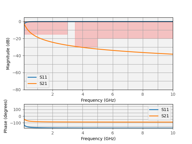
The optimized filter performance.
Discussion
The current method of optimization with differential weighting is better at consistently finding local minima especially with smaller population sizes. It still is far from perfect because the number of iterations are still large (too large for usage with FEM solvers) and it doesn’t modify the objective space enough to have gradient-based methods find the global minimum (which would be ideal).
However, it does introduce a simple numerical tool for improving optimizer performance when trying to generate filtering behavior.